| |
|
We have implemented 32-bit floating point operations (add, subtract and multiply) on the Cell Matrix. Doing so is relatively straightforward. Floating point numbers are stored as a mantissa (fractional point F) and an exponent E (multiplier). The number X is basically stored as a pair (F,E), where X = F * 2E (skipping a few minor details). Click here for more details on addition/subtraction or multiplication of floating point numbers.
Once you have floating point available, you can combine these into a floating point polynomial evaluator. Why evaluate polynomials? Because floating point polynomials are one way to compute scientific functions such as cos() and exp(). This is done using the Taylor Series expansion of these functions. A Taylor Series is basically a polynomial which is equivalent to the given function. The trick, however, is that such polynomials generally have an infinite number of terms. However, in many cases, all but the first few terms are extremely small, and thus don't have an appreciable affect on the polynomial's fnial value. For these cases, we can approximate the value of the scientific function by using just a few terms of the Taylor series (note that floating point numbers are often approximations: on most computers, the number 1/3 cannot be stored exactly, only approximated!).
Here is a movie of a polynomial circuit evaluating the exp() function (Copyright notice).
You can also view a more detailed, static image
here. The circuit works as follows:
|
| |
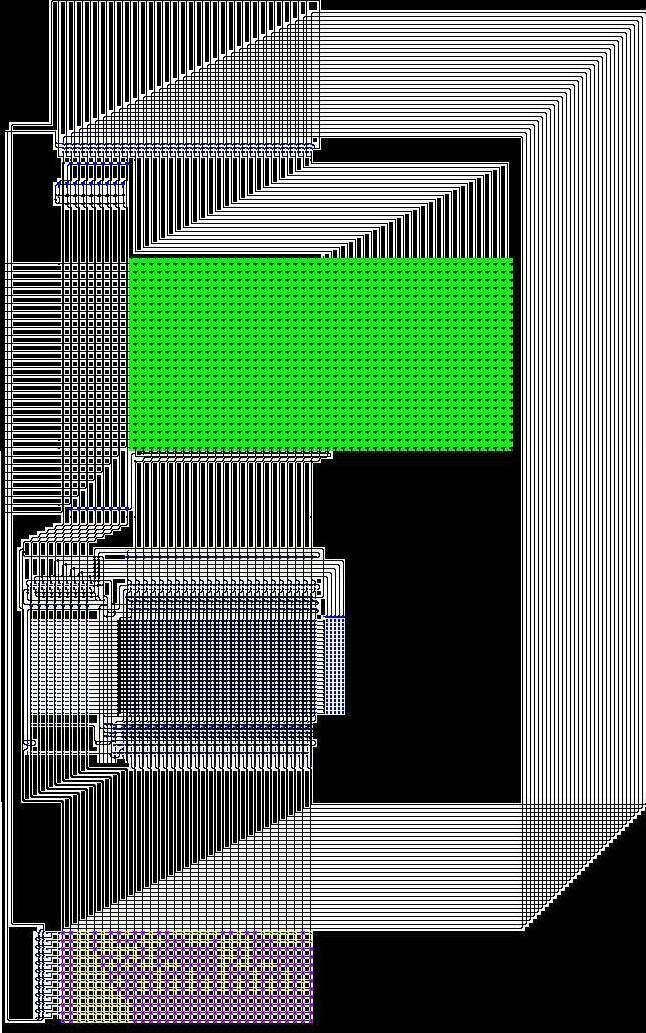
the number X at which to evaluate the polynomial is sent into the left edge of the circuit (the set of horizontal lines, about 1/3 down the left edge).
a set of polynomial coefficients is sent into the bottom of the circuit;
a register near the top of the circuit is initially cleared, and stored the running sum of the polynomial;
This running sum is multiplied by X, by the circuitry in the top half of the circuit (around the green block). To this product, a coefficient is added by the circuitry in the bottom half. The result is stored in the register, and this step repeats, again multiplying the sum by X and adding the next coefficient. After a fixed number of cycles, the process stops, and the register holds the final output value. Note that the circuit does not explicitly compute powers of X. Rather, it expands the polynomial into a different form, where it can be evaluated by a succession of multiply/add steps.
The purple/yellow block at the bottom of the circuit is where the polynomial's coefficients are stored. Each row stores one floating point coefficient, and these stored numbers are sent to the adder in turn.
In the movie, you can see the progress of the multiplier and adder blocks; the generation of successive constants from the bottom coefficient block; the feedback of each new sum at the bottom to the running sum register at the top; and the shifting of the fractional parts in the add/shift integer multiplier in the top half of the circuit (the jagged lines from lower left to upper right).
Note that a lot of cells are spent with simply wiring (for example, the wires that sent the adder's output from the bottom to the top of the circuit). This could be made more space-efficient, but for clarity, things have been left in a more easy-to-read layout.
| |
|
|
|
| |